Simple simulation and analysis

A quick and simple simulation to start with FRED simulations or to test a new installation can be run using a default setup. To get the default setup, just run FRED with an empty input file. All parameters are then set to their default value, as described hereafter.

1. Create a new folder, where the simulation is running, and enter to it:

$ mkdir fredSim
$ cd fredSim

2. Create an empty input file:

$ touch fred.inp

3. Run simulations:

$ fred

Default setup description

The default setup corresponds to a proton beam hitting a water box. The default field is Field_0 propagating along Z. There is a single pencil beam directed along the field axis and consisting of monoenergetic 100 MeV protons. The FWHM of the pencil beam is 0, i.e. it is a pin-like beam of perfectly aligned particles. The Phantom is a 4x4x10 cm³ box filled with liquid water. The scoring grid is made of 41x41x100 voxels. The phantom origin is at the Room centre, and the pivot point is at [0.5,0.5,0.0], i.e. it is centred in X and Y, and placed at Z=0. Propagation in the Field and in the Room is in vacuum. Hence, the protons are all entering the phantom with the initial energy of 100 MeV. FRED will track nprim=10000 primaries and score the deposited energy and the dose inside the phantom.

Simple analysis

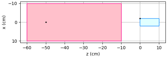
You can see the scene of simulation using a command:

$ sceneViewerFred.py

A scene corresponding to the default setup.

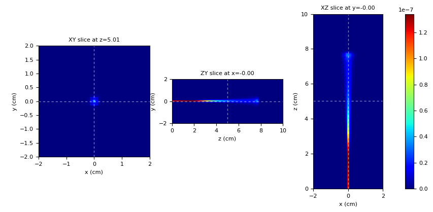
For instance, you can visualize the dose using a command:

$ mhd_viewer.py out/Dose.mhd

Dose map for the default setup (linear scale).

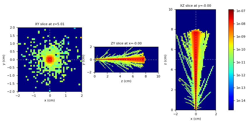
By pressing y you can change to scale of the color map to logarithmic.

Dose map for the default setup (logarithmic scale).

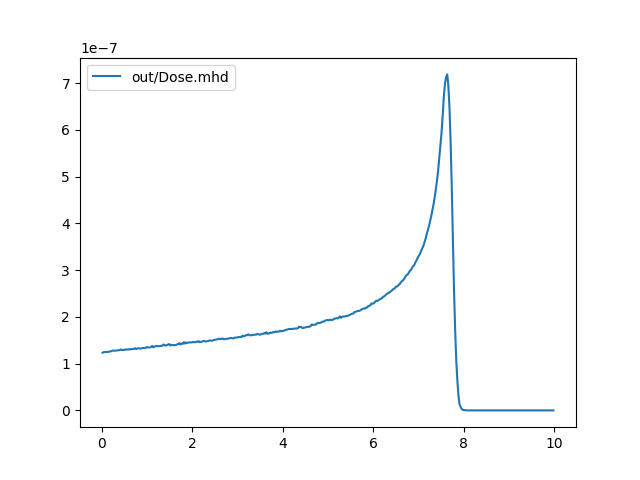
You can visualize the ddd (dose-depth-distribution) using:

$ mhd_sliceint.py out/Dose.mhd -p

A ddd for the default setup (protons 100 MeV).