Pencil beam in water phantom

A simple simulation of a single pencil beam in water. The setup and the method presented in this example can be used to validate and optimize the initial energetic parameter of the pencil beam.

Input file

The beam is defined by means of an emittance model with parameters corresponding to the beam sizes of 0.5, 0.3, 0.2, 0.4, and 0.8 cm (sigma) at distances from the isocentre of -20, -10, 0, 10 and 20 cm, respectively. The distance from the source to the isocentre and to the phantom is 40 cm. The dose is scored in a water phantom of size 10x10x20 cm³ with pixel size 1x1x1 mm³. The initial energy is defined as a Gaussian distribution with the mean energy of 150 MeV and FWHM of 5 MeV.

### Phantom ###
region<
    ID=Phantom
    O=[ 0, 0, 0 ]
    f=[ 0, 0, 1 ]
    u=[ 0, 1, 0 ]
    L=[ 10, 10, 20 ]
    pivot=[ 0.5, 0.5, 0 ]
    voxels=[ 100, 100, 200 ]
    material=water
region>

### Beam ###
field: 1 ; O = [0,0,-40]; L=[10,10,20]; pivot = [0.5,0.5,0.2]
pb<
    ID = 1
    fieldID = 1
    particle = proton
    Emean = 150 # Mean energy in MeV
    EFWHM = 5 # Energy spread as FWHM of a Gaussian distribution in MeV

    Xsec = emittance

    # the Twiss parameters corresponding to the beam sizes of 0.5, 0.3, 0.2, 0.4, and 0.8 cm (sigma)
    # at distances from the ISO of -20, -10, 0, 10 and 20 cm, respectively
    twissAlphaX=-1.235900963624794
    twissBetaX=8.3916636857885
    emittanceX=0.0034387868648755714

    emittanceRefPlaneDistance=40; # Field_1 origin is at 40 cm from ISO
pb>

nprim=1e6

Simple analysis

$ mhd_sliceint.py out/Dose.mhd -p

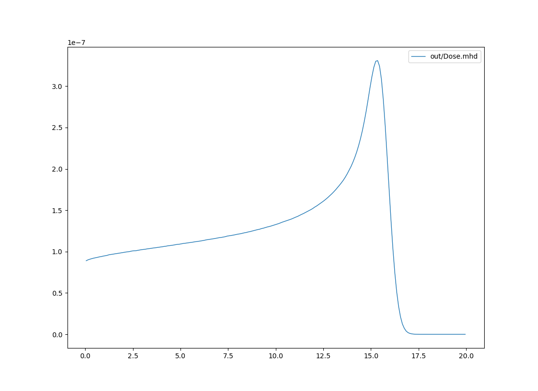
Bragg peak in water (integrated depth dose - IDD).