Sigma Squared model
This is a simplified and user-friendly model that allows to directly import spot size measurements into a Fred simulation. As the name is describing, the model is based on fitting the beam spot size using a second order polynomial, as described in the emittance model section:
Let’s take as a reference the case described by the following plot, showing the spot size measurements (blue stars) in the x direction taken at 5 different positions around the isocenter for a 100 MeV beam in a cyclotron facility.
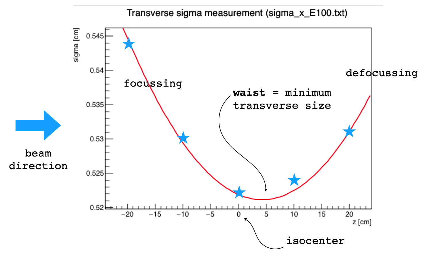
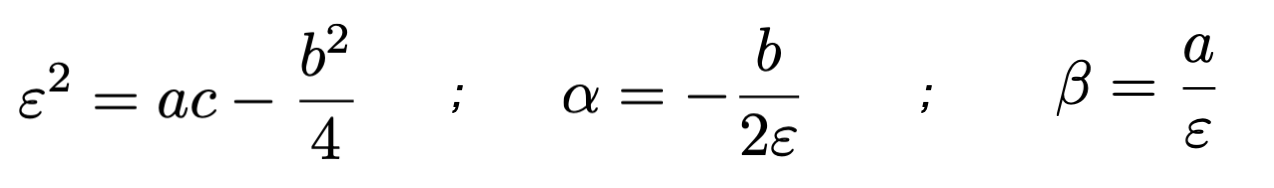
By fitting a parabolic function through the squares of the measured points
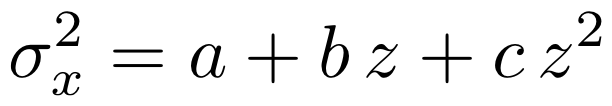
we can obtain the parameters needed for the emittance model
Example of a simple calculation in python using the measurements of previous Figure
from math import *
import numpy as np
import matplotlib
matplotlib.use('TkAgg')
import pylab as plt


zmeas = np.array([-20,-10,0,10,20])
sigmeas = np.array([0.544,0.530,0.522,0.524,0.531])

[[c,b,a],cov] = np.polyfit(zmeas,sigmeas*sigmeas,2,cov=True)

print('a=',a)
print('b=',b)
print('c=',c)

zmodel = np.linspace(np.min(zmeas),np.max(zmeas),400)
sigmasqr = a+b*zmodel+c*zmodel*zmodel

plt.ion()
plt.plot(zmodel,np.sqrt(sigmasqr),'-r',label='sigma squared model')
plt.plot(zmeas,sigmeas,'*b',label='data',markersize=10)
plt.legend()
plt.ylim(0,0.8)
plt.grid()
plt.xlabel('beam axis coordinate (cm)')
plt.ylabel('spot size (cm)')
plt.show()

input('return')
which gives in output
a= 0.27326425714285724
b= -0.0003427399999999939
c= 3.9535714285714174e-05
Important
In the previous example, the parameters have been obtained with respect to the isocenter position which is at coordinate z=0 cm along the propagation direction. Since particles are generated in the field FoR, we have to inform FRED of the distance from field origin to the isocenter in order to have the correct spot size evolution along the beam axis. To this purpose, we define D_ISO has the distance of pencil beam origin and the isocenter.
- sigmaSqrModel = [D_ISO, aX, bX, cX, aY, bY, cY]
D_ISO : distance (cm) from pencil beam origin to ISO center plane
aX, bX, cX : interpolation parameters for sigma_x as described above
aY, bY, cY : interpolation parameters for sigma_y as described above
parmeters for Y are optional: if not present, the values of X are mirrored
The input lines for source definition using the sigma squared model model syntax are
field: 1 ; O = [0,0,-55]; L=[10,10,20]; pivot = [0.5,0.5,0.2]

pb: 1 1 ; particle = proton; T = 100; sigmaSqrModel = [55,0.27326425714285724,-0.0003427399999999939,3.9535714285714174e-05]
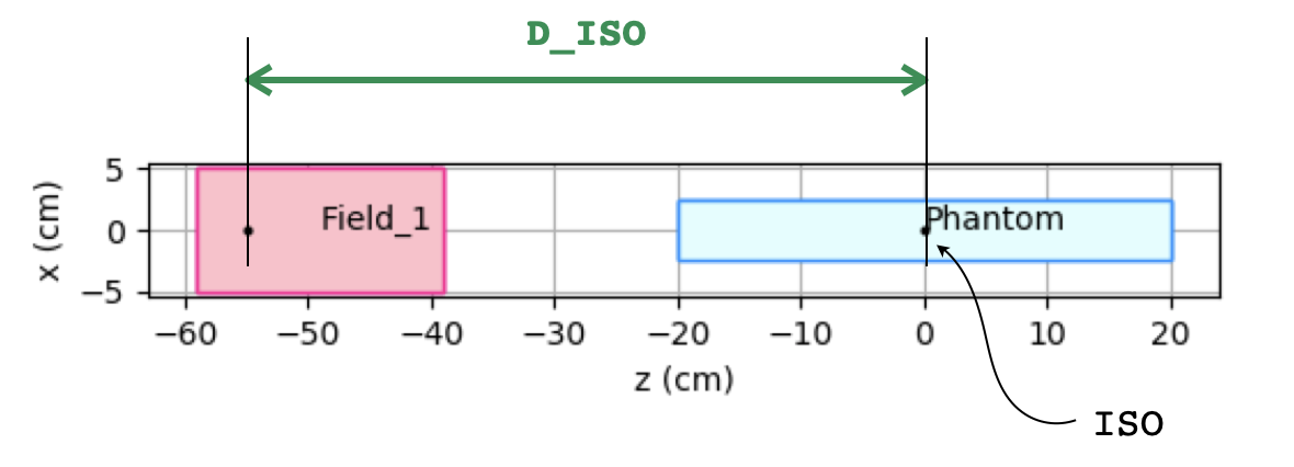
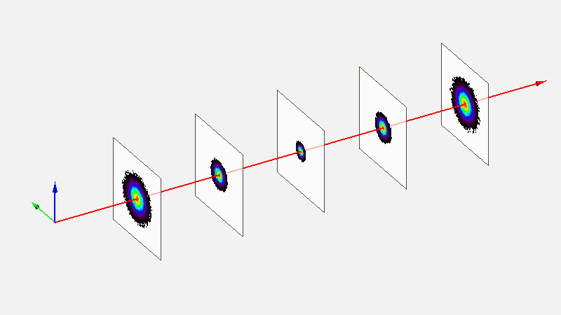
The evolution of beam cross section using the sigma squared model is represented by the following Figure